
Contents
- Overview
- Resources
- Approach
- Shape Classification
- Regularization
- Results of regularization
- Symmetry Detection
- Results of symmetry detection
- Curve Completion
Overview
-
Smoothy is a comprehensive pipeline designed for shape classification, regularization, symmetry detection, and curve completion. It is applied in real-world scenarios to recognize and transform hand-drawn shapes into precise geometric forms, even completing missing segments.
-
The pipeline employs a Convolutional Neural Network (CNN) to classify multiple polylines into specific shapes while accurately identifying the polylines corresponding to each shape. The model is trained on an augmented version of the QuickDraw dataset, covering 12 shape classes. The model is highly efficient, with a compact architecture comprising of just 0.6 million parameters, while still achieving a robust accuracy of 93.01% on the test set.
-
It uses shape replacement algorithms to replace the classified shapes with the regularized shapes making them geometrically correct. For curve completion, it detects potential occlusions, generates convex hulls for grouped polylines, and completes the curves using interpolation techniques.
-
It is applied in real-world scenarios to recognize and transform hand-drawn shapes into precise geometric forms, even completing missing segments.
Resources
The code for shape classification, regularization, and symmetry detection is implemented in the task-1.ipynb and the code for curve completion is in the task-3.ipynb notebooks respectively. The saved model for shape classification is in the shape_classifier.keras file.
For ease of access, you can use the following links to directly access the notebooks:
Input/Output Format
The input to the code is a CSV file containing the polylines. Each row in the CSV file represents a polyline, with the first column containing the polyline ID, second column is intentionally left blank, and the third column contains x coordinates and the fourth column contains y coordinates.
| Col_1 | Col_2 | Col_3 | Col_4 |
|---|---|---|---|
| 1 | 1 | 2 | |
| 1 | 2 | 3 | |
| 1 | 3 | 4 |
The code directly read the input.csv file and writes the output to the output.csv file. The input.csv file should be in same directory as the code.
Approach
Once we categorize the polylines into shapes, it becomes relatively simple to regularize the shapes and identify any symmetry within them.
In a nutshell, the approach can be defined follows:
- Classify the polylines into shapes using a
CNN model - Regularize the shapes
- Detect symmetry in the shapes
Shape Classification
Prediction Pipeline
Predicting any shape is quite complex since a shape can be depicted by one or multiple polylines. Therefore, it is impossible to ascertain which polyline corresponds to which shape. It is also important to consider that one polyline can be a part of multiple shapes.
In this ambiguous situation, we experimentally discovered the following approach to predict the shape:
-
First, we make classification on every single polyline. Now we consider the following three cases:
- If the polyline is classified as a shape other than
lineorcurvewithprediction probability(P) > 0.80, then we consider it as a shape and add it to final output. - If the polyline is classified as a
linewithprediction probability > 0.70and thehelper function 'is_line'which checks if a polyline is line based on the deviation from the actual straight line, returnsTrue, then we consider it as a line and add it to a set containing all lines. - All other polylines are considered as
curvesand added to a set containing all curves.
- If the polyline is classified as a shape other than
-
Now, the task can be broken down into finding shapes in the set of
linesandcurves. This simplifies the process as acurve can either be a curve, a circle, or an ellipse. To deal with this, the only option is to try all subsets of polylines. If we haveN polylinesthen we have2^N subsets. We can try all subsets and can select the predictions with maximum probability. However, creating all subsets is not feasible for large N and have large memory requirements. -
On further experimentation, we discovered that we can first try the subsets containing more polylines, i.e N, N-1, N-2, ... as they have a higher probability of being a shape. Thus, we first generate
thresholdnumber of subsets having polylines in decreasing order of N as they have a higher probability of being a shape. -
We then make predictions on these subsets and whenever a shape is predicted with a
probability ϕ > 'tline'for subset containing onlylinesandϕ > 'tcurve'for subset containing onlycurves, then we add it to the final output. It is important to note thattlineandtcurveare hyperparameters and can be tuned to get better results and the used values are also determined using hit and trial.- We now remove the polylines which are part of the predicted shape from the remaining set of polylines and recompute the subsets.
- We repeat the process until we have no polylines left or no prediction was made in the current iteration. If no prediction was made in the current iteration, we simply add the remaining polylines to the final output as lines or curves.
All the values of thresholds are determined experimetally.
The Model
We have used a Convolutional Neural Network (CNN) model which is trained on an augumented version of the QuickDraw dataset. The model is highly efficient, with a compact architecture comprising just 0.6 million parameters, while still achieving a robust accuracy of 93.01% on the test set.
The model architecture consists of four Conv2D layers with increasing filter sizes, followed by batch normalization and max-pooling layers to extract and downsample features. The model transitions to fully connected dense layers for classification, using dropout for regularization. The final output layer has 11 units, corresponding to the number of classes.
Before feeding the input to the model, the original input undergoes a series of transformations. These transformations include scaling, translation, normalization, standardization, resampling and Ramer-Douglas-Peucker algorithm. These transformations helps the model to learn the features of the shapes better and improve the classification accuracy while lowering the dimensionality of the input. Detailed explanation about each transformation can be found in the task-1.ipynb notebook along with the code.
Regularization
We have created a dedicated funtion to regularize each shape:
-
Rectangles: The code calculates the bounding box of the shape and constructs a regularized rectangle based on it, closing the loop to form a complete rectangle. -
Circles: The code calculates a bounding box, finds the center and average diameter, and generates a circular shape using trigonometric functions to create evenly spaced points around the center. -
Stars: The code identifies the bounding box, calculates the center and radius, and alternates between inner and outer radii to generate a regular star shape with evenly spaced points. -
Curves: The code smooths the curve using B-spline interpolation, producing a smooth curve with a specified number of points.
Due to limmitation of time, we cannot implement regularization for all other shapes. However, we smoothen all other shapes using B-spline interpolation with a lower smoothing factor to produce a smoother version of the shape.
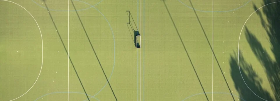
Results of regularization

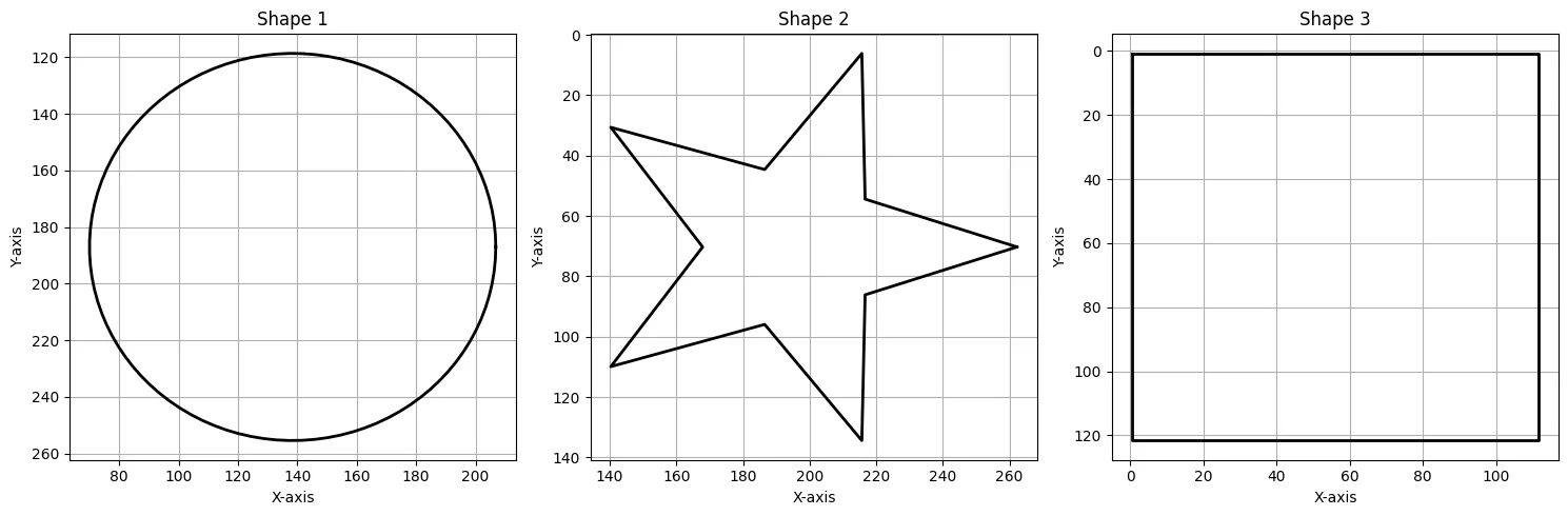

Symmetry Detection
We leverage the predictions made by the prediction pipeline to detect symmetry in the shapes. For all the geometric shapes, we can always say it will be symmetric with atleast one line of reference.
For example
- Circle: It is symmetric about any line passing through its center.
- Rectangle: It is symmetric about the horizontal and vertical lines passing through its center.
- Star: It is symmetric about the line passing through its center and any vertex of the star
- Ellipse: It is symmetric about the major and minor axis.
- Line: It is symmetric about its half.
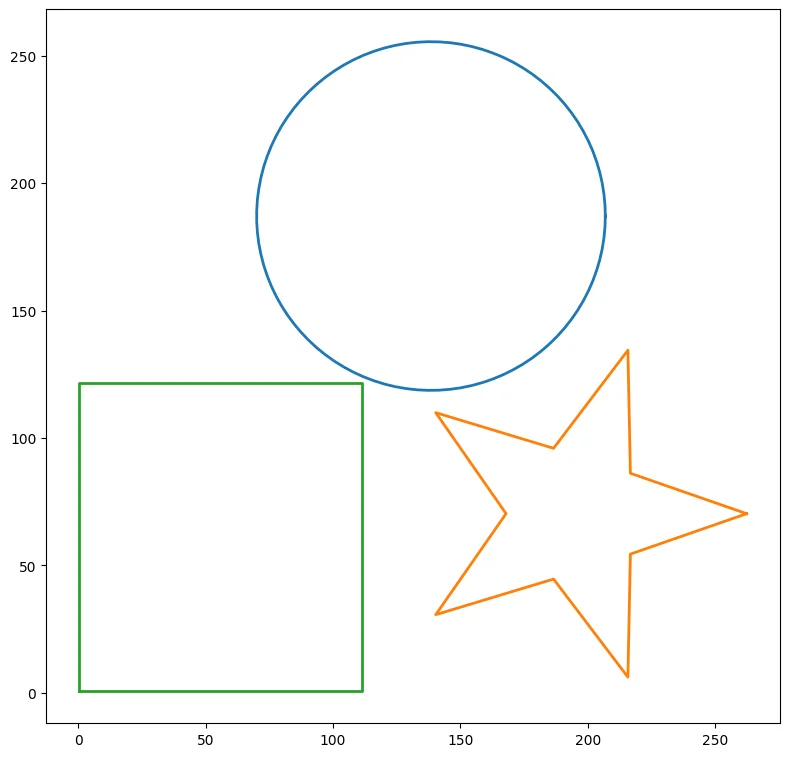
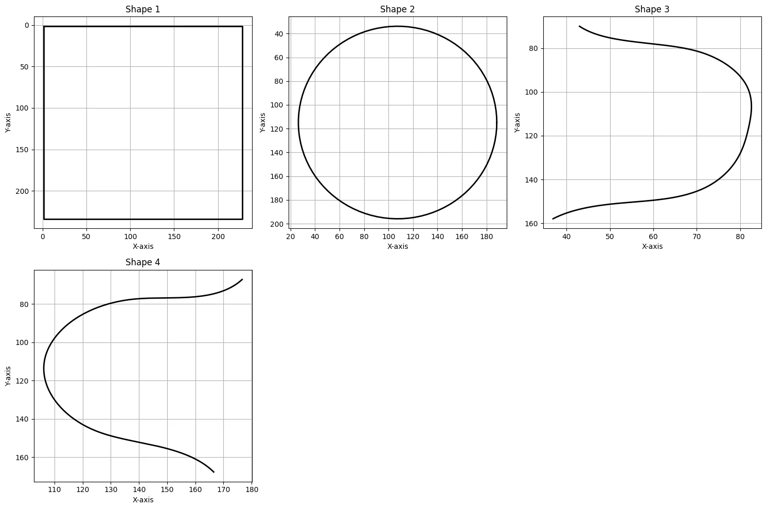
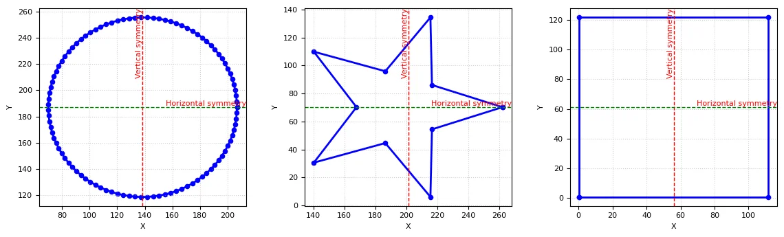
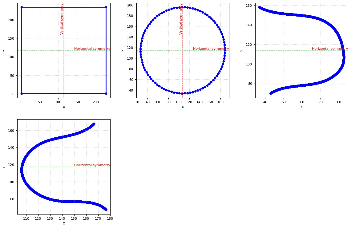
Now, the remaining task is to detect symmetry in the curves. To detect the symmetry in curves, we compare the left and right halves of coordinates around a mirror point. For vertical symmetry, we check if the x-coordinates are symmetric around the central x-value, while for horizontal symmetry, we check the y-coordinates around the central y-value. We use a threshold to determine if the maximum deviation is within an acceptable range to make more robust predictions.
Results of symmetry detection
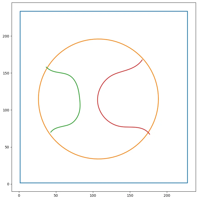
Curve Completion
After exprimenting a number of ways we have found that the following approach works best for shape completion:
-
The input data points are simplified using the RDP algorithm with a epsilon value of 2.0.
-
Occlusions are identified and the connectivity of the input data is checked using the aftermentioned steps:
- For each subset (which is essentially a set of points), the function tries to create a Polygon object using the shapely library.
- If the polygon is geometrically valid, it is added to a list of polygons.
- If the polygon is invalid, the 'make_valid()' function is used to correct it, and the corrected polygon is added to the list.
- The unary_union function is used to merge the polygons in the MultiPolygon into a single geometric entity (unified_poly) to combine overlapping or adjacent polygons into a single shape.
-
The shapes are completed by generating convex hulls for each subgroup.
-
The connectivity of the completed data is checked again and the status before and after completing shapes is compared.